Modern Music
Sentiment Analysis


Team Lyrics Lab

Kevin Buhrer, Michael Johns, and Scott Stephens

Overview

Did you know?

  • Word repetition in top charting songs has been increasing over the decades.
  • Over 55% of the artists in our data set had only one top charting song.
  • Offensive word use dramatically increased in the 1990s and continued to grow rapidly into the 2000s.
  • Over 15 songs are covers or remakes of songs already in the data set.

Music may tell us what the artist wants to say, but popular music tells us what the people want to hear. And that can tell us much about who they are. This project aims to discover the meaningful messages about cultures and their times, as revealed by the lyrics of popular music. It has long been recognized that studying a culture’s popular music can yield insight into its values and mood, but until recently analysis was confined to subjective examination of small samples.

In recent years, considerable effort has been devoted to studying and classifying two of the three basic ingredients of music: tones and rhythms. We studied the third ingredient, words, which have received comparatively less attention.

Studying song lyrics is different than general sentiment analysis of, say, a culture’s literature. Lyrics can have attributes that would be out of place in literature or formal prose, such as repetition, rhyming, and rhythmic delivery. Moreover, one might speculate that lyrics may have a higher tendency to be formulaic or even clichéd, making them more amenable to pattern analysis than prose generally.

Over most of the history of cultural musicology, research was hampered by the lack of available data. And when songs themselves became data stored on Compact Discs, the computing power necessary to conduct analysis was being devoted to other uses. Only recently has the abundance of storage and computational capacity made it feasible to study music’s messages empirically.

Trendy or Timeless?

Popular music is on the forefront of what the people consider new and cool, but it can also reflect shared values that are more persistent, even timeless. Leaving aside the ancient question of whether art imitates life or life imitates art, are there some concepts so firmly rooted in collective human belief systems that they remain constant across time? While a fully generalizable answer to that question may not be possible, some insights can be obtained from analysis of the content of the lyrics of popular music, and comparing them across time.

We chose to concentrate on the Billboard Year-End Top 100 Charts from 1970 to 2014, a corpus of 4500 songs spanning into 5 decades. By measuring, exploring, and analyzing the lyrics using a variety of techniques — including statistical, natural language processing, and machine learning — at multiple levels of abstraction, we were able to draw some preliminary insights, which will be highlighted throughout.

Screencast

An overview video is provided below. It has a running time of two minutes and is intended to provide an executive summary of the project. This site goes into far greater detail and we encourage you to keep reading.

It’s every generation throws a hero up the pop charts
— Paul Simon, "The Boy in The Bubble", Graceland (1986)

Artists

Can we learn more by looking at the artists or their words?

Artists can and do change over time, but almost all maintain a persona that is for the most part constant. Comparing the artists who have lasted, to the ones who did not can therefore tell us something about the enduring concepts in music. Of course, this gets complicated when an artist like Bob Dylan writes an iconic song celebrating change in one decade only to take the opposite view thirty years later. For the most part, we consider the persistence of an artist over a period of time a signal that the artist’s message continues to resonate with the populace.

For the times they are a-changin’
—Bob Dylan, "For the times they are a-changin’", For the times they are a-changin’ (1963)
People are crazy and times are strange
I’m locked in tight, I’m out of range
I used to care, but things have changed
—Bob Dylan, “Things Have Changed", The Essential Bob Dylan (1999)

Looking at the composition of the artists, we see that in any one year there are between sixty and ninety different artists represented in the Billboard Year-end charts, but over time a starkly different picture emerges. The vast majority of artists in our data have a small number of top songs—many only a single song—while a few artists have staying power and have many top songs.

Contributions by Artists

Most of the artists appeared in the corpus only once, but some occurred many times. Use the charts below to explore the distribution of artists and the number of their songs that ranked among the top. The charts increase visiblity of the artists with the most songs as you work through them.

Songs / Artists Distribution
 All
 > 2
 > 10

By contrast, we can also learn something from see how the top artists change over time. With the interactive chart below, you can see that Elton John ruled the 1970s, Madonna was the queen of the 1980s, with Michael Jackson in second place, and Mariah Carey led the 1990s, with Janet Jackson a distant second. In the early 2000s the television show American Idol propelled Kelly Clarkson to the top spot, and rap artists first began to be represented in numbers. Using the interactive chart below you can examine the productivity of the top artists for any time span ranging from the entire 45 years the data set down to a single year.

Most Succesful Artists Over Time

Use the chart below to filter the time period (click and drag to create a selection box). Use the table beneath to view a listing of the top 10 artists over the selected time period.

Top 10 Artists from 1970 through 2014

RankArtistTotal Songs# Chartings Years

What is it that these artists are saying? Here we take the collected lyrics of the top ten artists over the entire span of 1970-2014, and visualize their words according to how frequently they are used. There are some obvious patterns, such as the word “Love” appearing most prominently in every artist’s work except Michael Jackson’s. Maybe there are some more subtle patterns that can be discerned?

Words Clouds

Entire Corpus

Top 10 Artists (1970-2014)
 1. Madonna
 2. Mariah Carey
 3. Elton John
 4. Michael Jackson
 5. Rihanna
 6. Whitney Houston
 7. Janet Jackson
 8. Usher
 9. Stevie Wonder
10. R. Kelly

One theme often seen in popular music is rebellion. Not usually the kind of armed rebellion that led to the Battle of Gettysburg, but rather a rejection of (some) traditional values in favor of new ones. For example, Gil Scott-Heron’s 1971 cut “The Revolution Will Not Be Televised” has direct references to pop culture of the day and rejects them. Some credit the song as a precursor of modern rap and many artists (rappers and others alike) have referred to it in their own works. Taking on a broader scope than rebellion, we also see change as a common theme. Artists as diverse as Sheryl Crow, Bob Dylan, and Michael Jackson embracing change in different contexts.

I'm starting with the man in the mirror
I'm asking him to change his ways
And no message could have been any clearer
If you want to make the world a better place
Take a look at yourself, and then make a change
Michael Jackson, "The Man in the Mirror", Bad (1988),

While uses of the word change are readily available, is change really the most prevalent? Using the word frequency displays from above, one can conclude that love is at least among the most persistent themes in popular music, being measurably in common with prolific artists through the years. Again though, is love really the most prevalent? While a cursory review of top artists lyrics further clarifies our intuition that songs — and by proxy, artists — can be linked by lyrics, it does not fully settle the question of timelessness for all charting songs since 1970. With increased confidence, we pursued more rigorous techniques to gain deeper insights into the variety of perspective that have charted across the last five decades, the outcomes of which are presented in the sections to follow.

Data

Song lyrics offer an accessible corpus to analyze for topics and sentiments. Billboard provide numerous ranked charts that capture popularity of music. The charts consider both genre / sub-genre and artist and are backed by airplay, sales, digital downloads (since 2005), and streaming (since 2007). Though Billboard no longer supports a public API, Wikipedia preserves the lists. We have chosen Billboard’s US Year-End Hot 100 Singles as the foundation data source for this project, which has been maintained since 1951 (only top 30 available from 1951 to 1955).

Due to variations in song content if we were to cover the entire 60+ years of available chart data, we chose to focus on 1970 to the 2014, as 2014 is the most current year with year end charting. We were able to obtain lyrics from lyrics.wikia using their public API. We were also able to locate some partial data from a student named Samantha Stephens at HEC Paris who is doing her dissertation on environmental messages put forward by various artists. Samantha’s work filled in some lyric gaps, but not all. After accounting for instrumental music in the charts as well as other unavailable lyrics, the actual lyric corpus usable for text analysis was reduced to 4341 from the 4500 songs charted over the time period of interest.

Corpus Facts

The corpus covers 45 years of songs from the Billboard Year-end Charts. The charts give the top 100 songs for each year, yielding 4500 initial songs.

194 Multiyear Songs

Some songs remained popular for over a year: a total of 194 songs spanned more than more year. No multi-year song spanned more than two years and all occurred on consectutive years.

20 Instrumentals

Of the 4500 songs 20 are instrumental and are excluded from the lyrics analysis.

139 Songs Missing Lyrics

For 139 songs lyrics could not be obtained:

  • 36 due to licensing restriction
  • 103 have not been added to our lyric source, lyrics.wikia.

Word Count Reduction Motivation

As will be drawn out further in subsequent sections, lyrics can be quite repetitive. Using a raw, or straight-forward, count when the corpus includes a small number of songs which heavily repeat select words can skew certain analytics and measures if methods do not account for such repetition. An example effect would be using the raw count of each word to establish decade spanning nouns and adjectives in NLP. In this use, we want to understand and convey the diversity of songs using a word at least one time but do not want to allow any song with heavy word use to dominate the measure. For this, and similar purposes, we established a reduced corpus having the same number of unique words but only counting word appearances a maximum of one time per song. If a song had “baby, baby…”, baby would only be counted one time. At other times, repeating words use is of interest to our methods, such as the finding appearing in Word Use.

Adjective n-grams
Noun n-grams
  • Legend
  • Reduced n-grams
  • Non-reduced n-grams

Word Use

Linguists often examine the number of different words used in a text, called lexical diversity or simply, “vocabulary.” For most text, the use of a greater range of words is seen as a measure of superior articulation, but in music that may not be the case. Repetition has rhythmic and other cognitive function in music that renders comparison to the lexical diversity of prose pointless. We can, however, compare a song’s vocabulary to that of other songs, and in particular can see how lexical diversity has changed over time. One could argue that songs with more distinct words are intended to contain more complex meaning, while songs with more repetition are more likely to be using the words as an aural device- that is, for their sound value rather than their semantic content. The words oh, oo, la, and yeah are examples of words more likely to carry sound than meaning.

Here we depict the changes in word count and lexical density over the years. It appears that the words per song has mostly increased over time, though decreasing since the turn of the century. And we do see declining lexical density, indicating increased repetition. More words with less to say.

Lexical Diversity
Word Repetition

Word Counts

Overview
Raw Words
Unique words
  • Legend
  • All words, Decade Trend
  • All words, Year Trend
  • Unique Words, Decade Trend
  • Unique Words, Year Trend

NLP: Natural Language Processing

Word Variation

To put a finer point on the word usage inquiry considered in Word Use, we consider that words, like styles, have differing popularity levels at different times. The words contained in song lyrics were separated into adjectives and nouns with the other words being discarded. The words were evaluated for how often each appears per decade, understanding that the “decade” labeled 2010 is for only half a decade (2010 through the end of 2014). Again we see that love is the most dominant and persistent theme, though time, baby, and girl begin to eclipse love starting in 2000.

Top Adjectives Over the Decades

1970s
1980s
1990s
2000s
2010s

Top Nouns Over the Decades

1970s
1980s
1990s
2000s
2010s

Timeless Words

A large number of the words found in popular songs don’t make it from one decade to the next. Here we display the number of each type of word having lifespans from one to five decades, and also display the words spanning or enduring across all five decades. This inquiry uses the reduced vocabulary as described in Data to mitigate the skewing effects of heavy repeated use of the same word in any given song.

Adjectives Spanning Decades
5-Decade Spanning
Decade Distribution
Nouns Spanning Decades
5-Decade Spanning
Decade Distribution

What is a Hypernym?

In general, a hypernym is a superordinate word or phrase (Wikitionary). In the context of this study a hypernym is a pair of synonyms that share a common parent. They are used to reduce the vocabulary even further.

Vocabulary

Beyond splitting out parts of speech, we also recognized that words are related in various ways and wanted to collapse similar meaning words to a common one for analysis and measuring. We chose synonyms and hypernyms to draw together semantically similar peers (synonyms) and then synonym children to their common parent (hypernyms), accepting the tradeoff of vocabulary consolidation for a slight loss of semantic precision. The primary use in mind for shrinking vocabularies, was to improve the performance of our machine learning techniques. Here is the results for shrinking the nouns first by synonym and then shrinking again by synonym with hypernym replacement. More details on how we established the vocabularies are available in Vocab-Consolidation and Vocab-Shrunk Notebook.
Vocab Version Vocab Name # Unique Nouns Words Consolidated Reduced Word Use (1x max per song)
Initial Word Vector 5138 0 35,120
Shrunken-1 Synonym Vector 3230 1908 7,644
Shrunken-2 Synonym With Hypernym Replacement 3215 1923 494 hypernyms in 7,644

Synonyms

We used Natural Language Tool Kit NLTK, specifically its Synset API, to build synonyms for nouns and adjectives.

Adjective Synonyms

Here is an example of adjective synonym pairs and how they were shrunk, with “crimson” being the first common synonym for both “scarlet” and “ruby”:

To better understand the effects of synonyms, we measured the total reduced or unique song uses of adjective synonym over the decades, shown to the left. Below, we measure those shared, i.e. “timeless”, adjective synonyms appearing in all decades.


Noun Synonyms

Here is an example of noun synonym pairs and how they were shrunk, with “chatter” being the first common synonym for “yack”:

We also measured the total reduced or unique song uses of noun synonyms over the decades, shown to the left. Below, we measure those shared, i.e. “timeless”, noun synonyms appearing in all decades.


Hypernyms

We used NLTK Synsets to collapse synonym child pairs to their less-granular semantic parent or most common peer, based on Synset rules.

Adjective Hypernyms

Here is an example of adjective synonym pairs were shrunk to a common hypernym, with “bare”, “naked”, and “nude” shrunk to hypernym “bare”.

To better understand the effects of hypernyms, we measured the total reduced or unique song uses of adjective hypernyms over the decades, shown to the left. Below, we measure those shared, i.e. “timeless”, adjective hypernyms appearing in all decades, as well as those appearing 5 or more times, even if not in every decade.


Noun Hypernyms

Here is an example of noun synonym pairs being shrunk to their common hypernym, with “aim” and “intent” being shrunk to “purpose”.

We also measured the total reduced or unique song uses of noun hypernyms over the decades, shown to the left. Below, we measure those shared, i.e. “timeless”, noun hypernyms appearing in all decades, as well as those appearing 5 or more times, even if not in every decade.


Vocabulary Shrinkage

An effect of shrinking vocabularies with synonyms and hypernyms is that the vectorization of the words for corpus analysis can produce derived empties, in addition to the missing lyrics described in Data. The table below shows the further lyric eliminations needed in order to run noun analytics such as demonstrated in Prediction.

Category Why Empty? # Empties Corpus Size: 4500
Vocab Initial (noun vector) 220 4,121
Vocab Shrunken-1 (synonyms) 16 4,105
Vocab Shrunken-2 (synonyms w/ hypernym replacement) 0 4,105

Offensive and Slang Words

Clean Versions

Radio edits are becoming increasingly common. A recent NPR article from from November 8th, 2015 entitled The Art Of The ‘Clean Version’ discusses how many outlets address offensive language and their varying techniques.
When I spoke with Guerini [Radio Disney], he said almost half of the more than 50 songs on rotation at the time had been edited.
—Priska Neely

Until the end of the 1990s, vulgar or obscene lyrical content was almost entirely absent from the top selling songs. Even artists as avant garde as Frank Zappa toned down some of their lyrics to find commercial success. In late 1973, Zappa released the album Overnite Sensation, containing a cut “Dirty Love” with explicit reference to bestiality. Another Zappa album, Apostrophe, quickly followed in early 1974, whose most offensive lyric was “don’t eat the yellow snow.” Overnite Sensation, with its explicit lyrics, received no airplay Apostrophe became popular, peaking at no. 10 on the album charts.

Under the regulations of the Federal Communications Commission, vulgar or obscene language is not permitted in material broadcast over the publicly owned electromagnetic spectrum. Artists still used the words, but the result was no radio play, or in some cases altered, sanitized versions for radio. As long as access to the mass market was dependent on radio play, musicians who wanted to reach that market kept the lyrics within bounds.

Outside of the broadcast context, efforts to ban certain words had the opposite of their intended effect. Hardly anyone had heard of 2LiveCrew before they were banned in Miami for using offensive language. Sales took off overnight.

The digital revolution changed everything, especially music. According to Public Enemy’s wikipedia page, they were the first to release an album in the MP3 format. Rapidly the distribution channels became less and less dependent on radio, and the composition of the vocabulary formerly known as offensive began taking on the structure we see today. As is visualized below, while offensive language was in check for the majority of songs charting in the 70s and 80s, the introduction of new channels beyond radio, coupled with reduced cultural morays resulted in a steady climb in offensive language use in the 90s forward to current music in the 2010s.

  • Legend
  • 1970
  • 1980
  • 1990
  • 2000
  • 2010

First Appearance of Offensive Words

  • 1970
  • shit from "American Woman" by The Guess Who
  • 1971
  • dick from "Theme from Shaft" by Isaac Hayes
  • 1973
  • bullshit from "Money" by Pink Floyd
  • 1975
  • pussy from "Killer Queen" by Queen
  • 1977
  • bitch from "Rich Girl" by Hall and Oates
  • booty from "Dazz" by Brick
  • 1983
  • ass from "Little Red Corvette" by Prince
  • 1987
  • butt from "Bad" by Michael Jackson
  • 1992
  • ho from "Baby Got Back" by Sir Mix-a-Lot
  • niggaz from "People Everyday" by Arrested Development
  • 1993
  • motherfucker from "Nuthin' but a 'G' Thang" by Dr. Dre
  • pimp from "Rebirth of Slick (Cool Like Dat)" by Digable Planets
  • 1994
  • whore from "U.N.I.T.Y." by Queen Latifah
  • 1996
  • pimpin from "Tonite's tha Night" by Kris Kross
  • 1999
  • cock from "Can I Get A..." by Jay-Z
  • titty from "Back That Azz Up" by Juvenile

Topic Modeling

We now move beyond the use of specific words used in isolation. Topic modeling techniques seek to identify the subject matter of a body of text by evaluating context or more precisely collocation of words. These methods — Latent Semantic Indexing (LSI) and Latent Dirichlet Analysis (LDA) — calculate the frequency with which words appear together combining these measures to produce groups of words that are likely to indicate a topic contained in the text. The technical details of these processes are contained in ipython notebooks referenced by our Master Process Notebook that conduct analysis on the entire data set on data partitioned by decade and on data partitioned by genre. We obtained 90 topic estimations for LDA routines and 300 for LSI, and repost only a small fraction of the results in the table:

LDA Analysis by Decade and Genre

0 1
all decades and genres hitta, day, shit, ride, finger, trigger love, baby, girl, time, thing, night
decade: 1970s schoolgirl, glare, passin, monsoon, goner gasp, broken, grate, guitar, pickin
decade: 2010s serenity, spinnin, iceberg, susie, redhead wrist, whack, mam, jail, order
genre: country music thank, mistake, sand, ticklin, letter redneck, kid, hell, church, laugh
genre: hip hop music game, gold, hide-and-seek, rap wish, arm, dynamite, sound, relaxin

Similar results were obtained using LSI, and by using both LDA and LSI on synonym-reduced and hypernym-reduced Vocabulary sets. Ultimately, the results of topic analysis have to interpreted subjectively; in this case the results for all years and genres combined seem to have more semantic value than the subsets by genre and decade, both of which yielded much smaller sample sizes. For example, topic zero for all decades and genres seems to indicate a violent theme, while topic 1 reinforces the central observation that love is the most timeless value reflected in music.

Prediction

Top 50 versus Bottom 50

While we understand that a song’s lyrics are not generally causal to where a given song might land on the charts, we had a hunch that there might at least be a correlation between a song’s position and its lyric content that we could model, train, and ultimately do some prediction. Having already explored Topic Modeling with Latent Factors as shown in the previous section, we wanted to separately focus on supervised learning techniques that would be more readily interpretable. Ultimately, we landed on predicting the ‘Top 50 versus Bottom 50’ positions on the 2014 charts, a balanced set of positives and negatives, also offering a binary prediction, where positives values indicate ‘In the Top 50’ and negative values indicate ‘In the Bottom 50’. We also wanted to again leverage the cluster computing framework Spark as we had used previously in establishing the Vocabularies. 
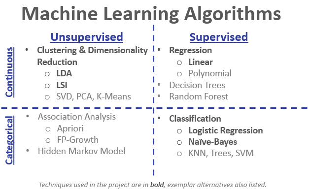
For prediction, we were interested in its Machine Learning APIs. After some trial, error, and tuning, we used Spark’s Pipeline API to apply Logistic Regression learning algorithm, or estimator, which turned out to be a solid choice for this exploration as it favors binary, balanced data. More in-depth information for our approach and results can be found at Vector Ensemble Notebook in addition to more cursory information in the project Master Process Notebook.

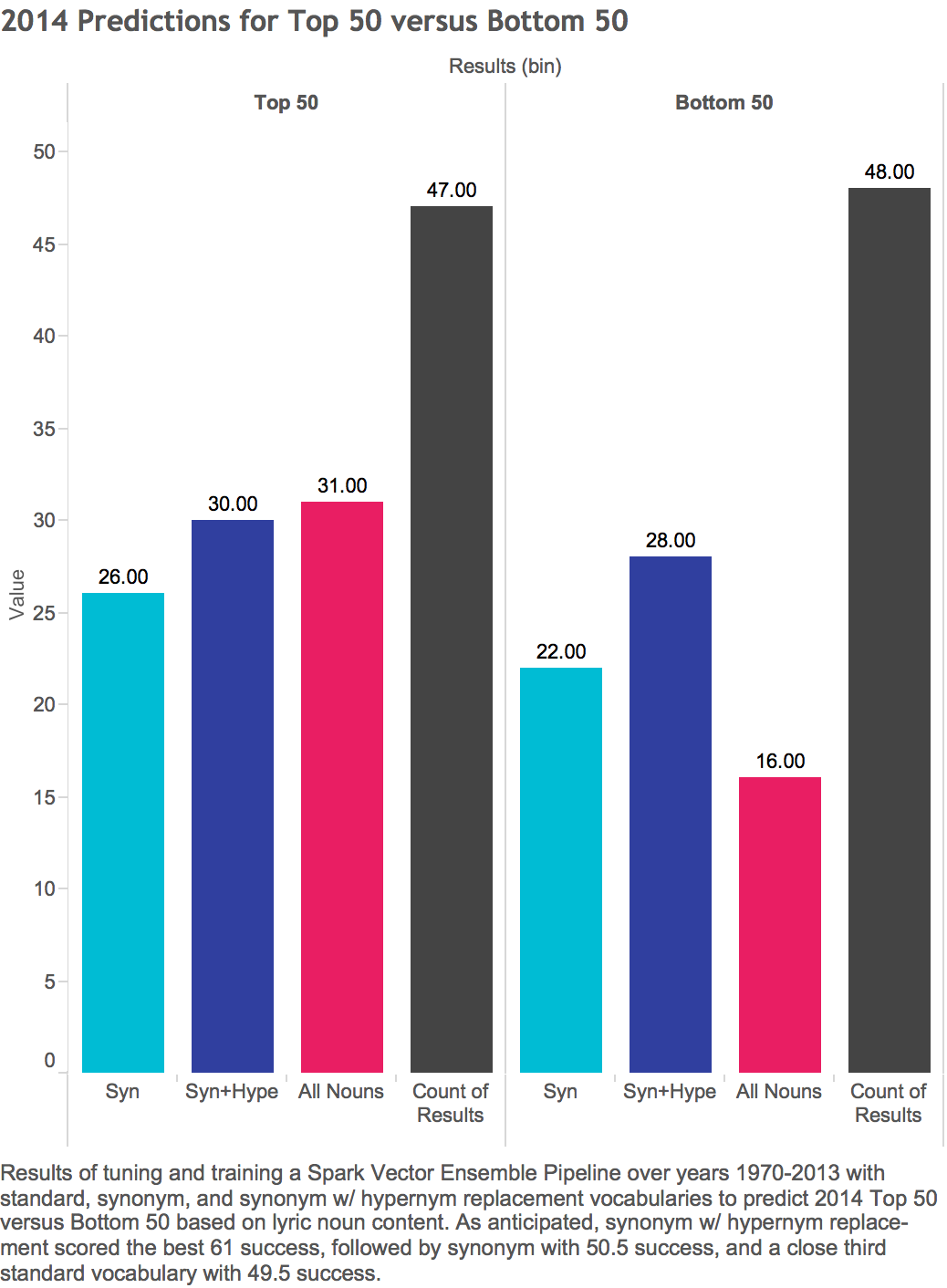
First, we tuned and fit models against noun vectors derived from all 3 Vocabularies — Initial, Shrunken-1, and Shrunken-2 — training on all data from 1970-2013 using the tuned hyperparameters. Then we predicted ‘Top 50 versus Bottom 50’ exclusively for 2014 using the same models derived from the 3 vocabularies.
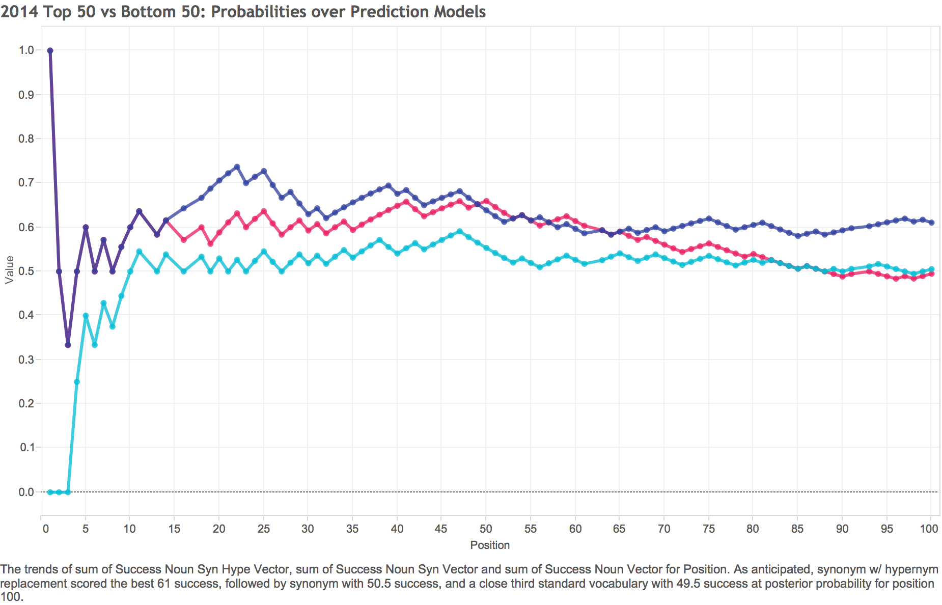
 
  • Legend
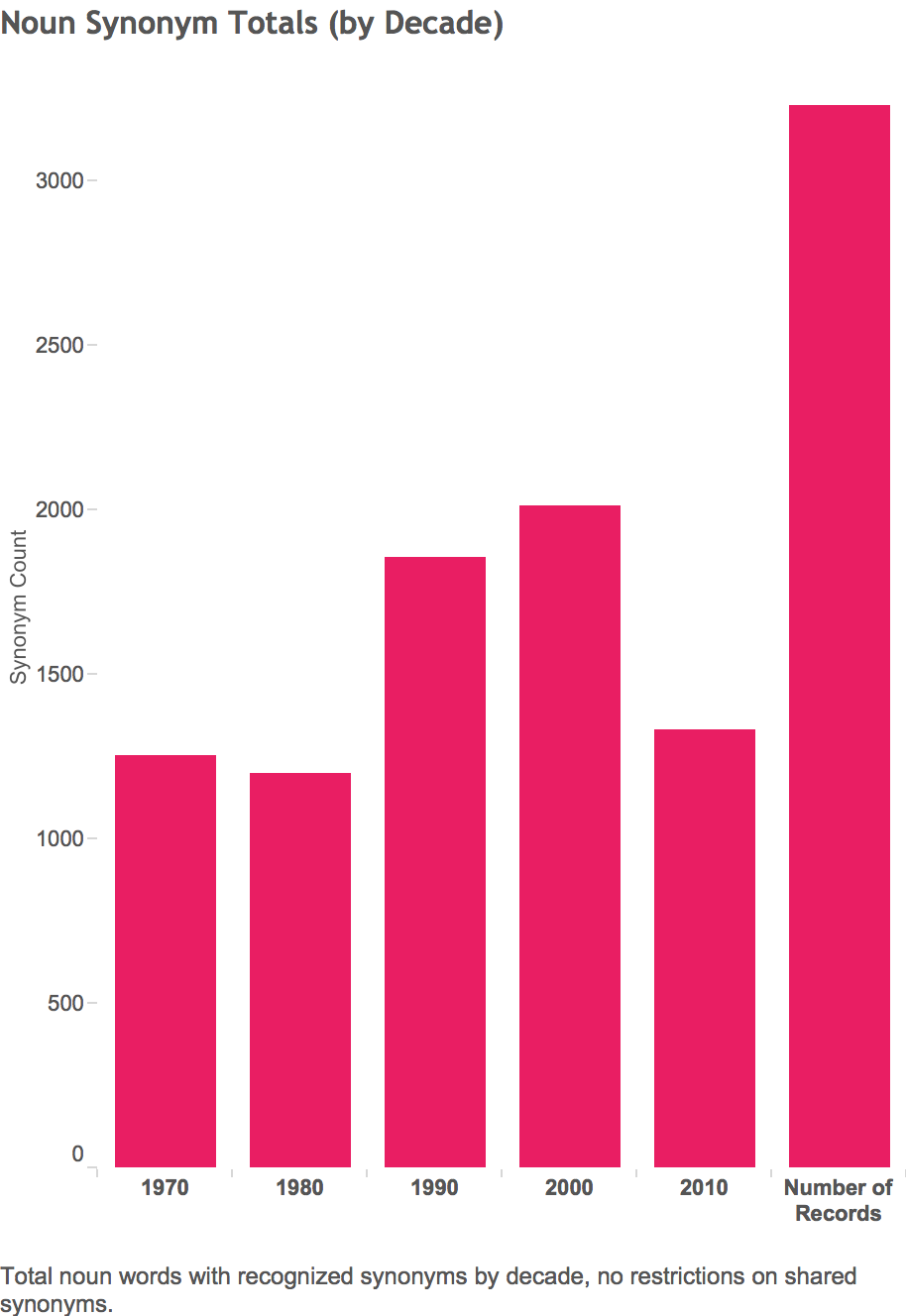
  • Nouns Synonym with Hypernym replacement
  • Nouns Synonym
  • Nouns

Prediction yielded the results shown in the table below. Note: only 95 of 100 songs in 2014 had populated noun vectors for all three vocabularies.

Vocabulary Posterior Percent Hits Misses
Initial (Nouns) 49.47 47 48
Shrunken-1 (Nouns Synonyms) 50.53 48 47
Shrunken-2 (Nouns Synonym with Hypernym Replacement) 61.05 58 37

At least to the degree that lyrics and position are correlated, the results of predicting the top / bottom splits are consistent with our intuitions. Initial vocabulary (vectorized to allow only each unique noun 1x max per song) was the least performant, slightly improved upon by model fit to Shrunken-1 (nouns with synonym replacement, also vectorized using same reduction rules as Initial), then a significant performance gain realized by Shrunken-2 noun vocabulary (synonyms with hypernym replacement, vectorized using same rules). Shrunken-2 correctly predicted 58 of 95 non-empty lyrics in 2014.

Phrase to Genre Prediction

Our final analytical technique uses a classifier to predict the genre that an ad-hoc, snippet of text is most likely to have come from. For this we use the Natural Language Tool Kit NLTK Python library and its Positive Naive Bayes Classifier module. We split the data into a training set and a testing set, and for each of the top 15 genres constructed a classifier using songs identified with the genre as the positive examples, and all other songs in the training set as negative examples.

For each included genre, a prior probability is calculated by calculating the relative frequency of songs within that genre in the training set multiplied by 0.097, the number of genres divided by the total number of songs. To see whether the choice of prior influences the quality of the model's predictions, the process is run with several other values for the prior, which are uniform and arbitrarily set. In the table, the "v' stands for a variable prior based on the genre-specific calculation; the others are uniform, meaning the same prior was used regardless of the relative frequency of songs in the relevant genre.

0.5 0.2 0.3 0.1 0.05 0.01 0.02 0.097
true positive: 1102 385 642 221 152 49 65 106
false positive: 6370 1837 3199 873 330 73 127 169
false negative: 496 1234 1003 1449 1492 1625 1636 1511
true negative: 4527 9039 7651 9952 10521 10748 10667 10709
Right/Total 0.450 0.754 0.663 0.814 0.854 0.854 0.858 0.865
Results
Total Positive: 1598
Total negative: 10897
Pct Positive: 0.128

These results indicate that the data are highly unbalanced in the negative direction, and indeed a simple baseline that always predicts negative would have a success rate comparable to the best prior's success rate, which was the variable prior based on the genre's overall prevalence.

Inspired by the adage that "all models are wrong, but some models are are useful," we resort to the obvious deployment of this battery of classifiers: Can it match arbitrarily chosen text to the genre from which it would come? These results suggest the answer is a qualified yes.

InputResponse
'how about we dance first' Dance Music
'beat the bitch with a bat' Hip hop Music
'you know i love you forever and ever'  Soft Rock
'gun shoot baby' Hard Rock
'gun shoot' Hard Rock
'woman left me, took my truck' Country Music
To add your own words or learn more about our approach, see the Positive Naive Bayes Classifier notebook.

Conclusion

In this project, the Lyrics Lab team employed powerful tools of data science to myriad experiences and ideals as articulated in lyrics, to approximate how lyrics express what it means to be human.

Music is the vernacular of the human soul
— Geoffrey Latham

We applied a number of statistical, natural language processing, and machine learning techniques to gain insights into the content of modern music lyrics. In the matrix below, we indicate which machine learning algorithms we implemented, much of which was presented in previous sections, though additional work was not presented for brevity. However, given the complex and nuanced nature of text analysis, there is much more we would have liked to explore for this project, given more time. The matrix below also indicates a sampling from the many other techniques available that might serve useful to obtaining a deeper understanding of modern music.

Adapted from an example graphic found here.

Here are primary guiding questions for the project which we approached to varying degrees of success:

Here are secondary questions, some of which the project assisted in answering:

While we explored a fair number of statistical and natural language processing techniques and approached a number of our guiding project questions, there is always opportunity for more exploration given the multifaceted nature of music, to include any relevant machine learning methods we were unable to apply given the duration and nature of the project. Some obvious places for further exploration begin with expanding the data set. Whether it be in terms of time frame; by using the Billboard Top 100 weekly charts; or including other data sources regarding radio plays, albums sales, or social media mentions. Other interesting directions would include isolating artists and further determining how consistently each abide their lyrical messages, isolating geographic / subculture message preferences, and correlating music trends to broader cultural trends. Finally, implementing song and artist recommenders based on lyric content would be very beneficial.

If you want to get a more behind the scenes look at what we have done, please start with our Master Process Notebook which lightly summarizes and links to various thread of exploration, also captured in ipython notebooks, undertaken by our team in the course of this project.

Perhaps the groundwork we have laid can assist in your research goals. If so, please contact us.